Large multidimensionaL Optimisator and Visualisation Explorer

            Yanxue Wang1, Madeh Sajjadi2, Abhishek Joshi3, and Sinuhé Perea4
1 Helmholtz-Institut Erlangen-Nürnberg für Erneuerbare Energien,
2 Institute for Advanced Studies in Basic Sciences,
3 Brandenburgische Technische Universität Cottbus,
4 Max-Planck-Institut für Kolloid- und Grenzflächenforschung;
                                            e-mail:sinuhe.perea@mpikg.mpg.de.

Abstract: As the marginal cost of information continues to decrease with the rise of virtual environments and digital technologies, traditional pen-and-paper graphs are becoming insufficient in daily research routine. Instead, abstract frameworks that manage large datasets, driven by statistical analysis or automated learning methods, are gaining prominence. However, there remain certain scenarios, particularly in exploratory research, where simple visual representations can provide initial momentum and valuable insights during the preliminary phases of studies or when modelling tools are limited. This article introduces a suite of functions developed within the Mathematica environment, designed for straightforward data visualisation and prediction in higher (yet manageable) dimensions. The suite includes simple histograms and correlation analysis, parallel axis plots, pseudo four-dimensional input and singular output visualisation, and iterative optimisation processes that extrapolate relevant novel manifolds for exploration. The suite is tested against three heterogeneous datasets: energy efficiency in residential buildings, abalone age prediction from physical measurements, and the optimisation of hybrid organic-inorganic solar cells.

---

Introduction

A good rule-of-thumb principle in Science is avoid forgetting the geometrical intuition in what you do. The appearance of hidden correlation may be ignored with simple visual inspect of the raw data obtained in the experiment and can potentially lead to longer computation times and obscuration of the obtained results. Data-driven techniques are built to surpass this issues with the corresponding optimisation and built-in tolerances that, unfortunately, rarely pop-up in the final results, if not explicitly asked. Then, a simple preliminary visualisation of the obtained results can be extremely useful when the objective is still unclear in exploratory research to avoid taking a wrong data-driven direction, or a simple model is sought initially.

Conventional languages as Python, MATLAB, Origin, or Mathematica are slowly introducing built-in features [A-D] enabling a better understanding of the raw multidimensional data acquired. But additional functionalities could be generally included, such as pseudo-visualisation of the simplest cases (between four and seven dimensions), initial data cleaning of outliers, or basic prediction models based on gradient descent optimisation. To this end, in this article, we represent a simple toolbox for higher dimensionality analysis LLOVE (Large multidimensionaL Optimisator and Visualisation Explorer) for the Mathematica language that includes easy functional scenarios that enables both inexperience users "plug & play" usage and an open code with introduction and explanation for easier customisation and additional further modifications.

In particular, in this tutorial, we are set to describe here six of its tools: histograLL, doubLLe, correLLAtion, paraLLel, baLL, and umbreLLa that jointly enable basic operations for data analysis in the shape of an interactive dynamic notebook that will be shown for three selected datasets, without a-priori knowledges about them, with a data-driven perspective: The first one will correspond to simulated building's energy efficiency from [E], abalone age estimation from physical measurements [F] from the Marine Resources Division (University of Tasmania) openly available thanks to the UC Irvine Machine Learning Repository, and SPINBOT perovskite solar cell optimisation [G] from a recent HI-ERN project, currently on press. They are referred in the following as energy.csv, abalone.csv and niox.csv, respectively, and include the different featured measurements as columns, with its corresponding header.

The file energy.csv correspond to the topic of energy performance of buildings (EPB) obtained with the software Ecotect (from Autodesk Inc., discontinued from 2023), formally with ten columns, the first seven are related to features of the building such as relative compactness, surface wall, and roof areas, overall height, orientation, glazing area and its distribution -compass rose (labelled X1-X8, ) and heating and cooling loads (Y1-Y2), for 768 different simulated structures.

For its part, the file abalone.csv includes another set of nine dimensions displayed in columns corresponding to properties of the marine snails such as sex (masculine, feminine, and infant), diameter, height, weight (total, shucked, viscera, and shell) and number of rings (that are proportional to the age of the haliotis), with a total of 4177 different organisms. The study was designed for aiming towards faster and non-invasive method for estimating the age of the snail without opening the shell itself which caused damages to the animal [H]. The relevance of this research is founded on the major alimentary industry around it in Australia, and the correct interpretation of its maturation and idoneity for human consumption results a key characteristic.

Finally, niox.csv is represented by ten variables: sample number, NiOx concentration, dropping time (T1), dropping volume (V1), dispense speed (S2), high-speed spin (S3) are the inputs of the samples and Jsc (circuit current density), Voc (open-circuit voltage), FF (filling factor) and Pmax (converted efficiency) correspond to the outcomes of the perovskite solar cells and including 144 elements consecutive measured using a automated device acceleration platform, to try to surpass the limitations on operator abilities and particular lab conditions and increasing steadily the current efficiency figures in pervoskite community trying to reach silicon or tandem cases.

---

Toolbox description

Basic histograms and correlations

Although no additional packages are needed, the initial step to load the files is place them in the same folder as this notebook and then evaluating the next cell to set the current environment in the local directory of this file:

SetDirectory[NotebookDirectory[]]

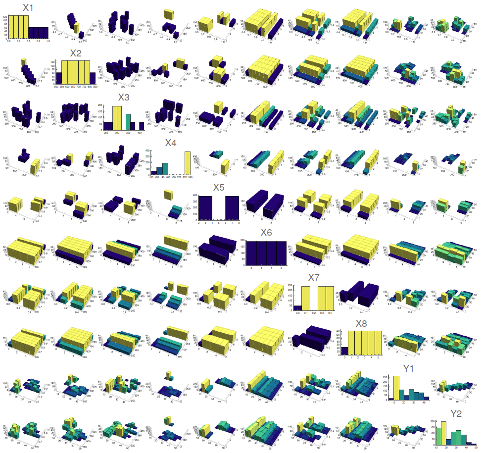
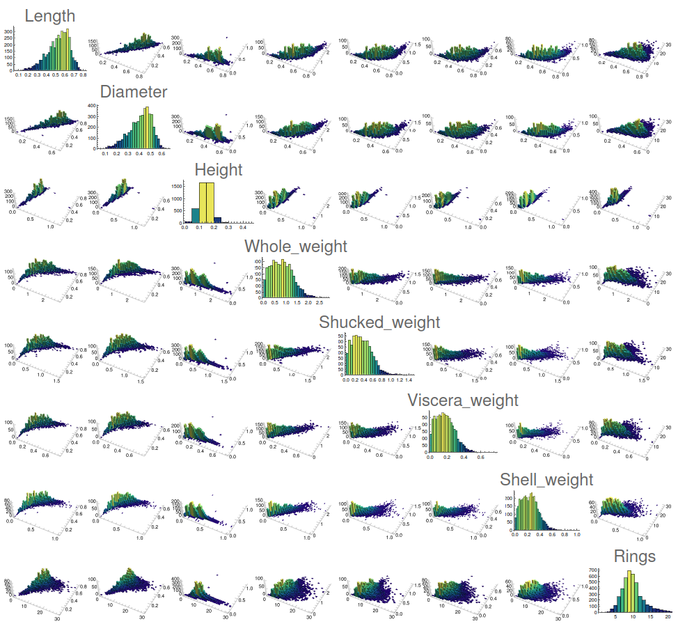
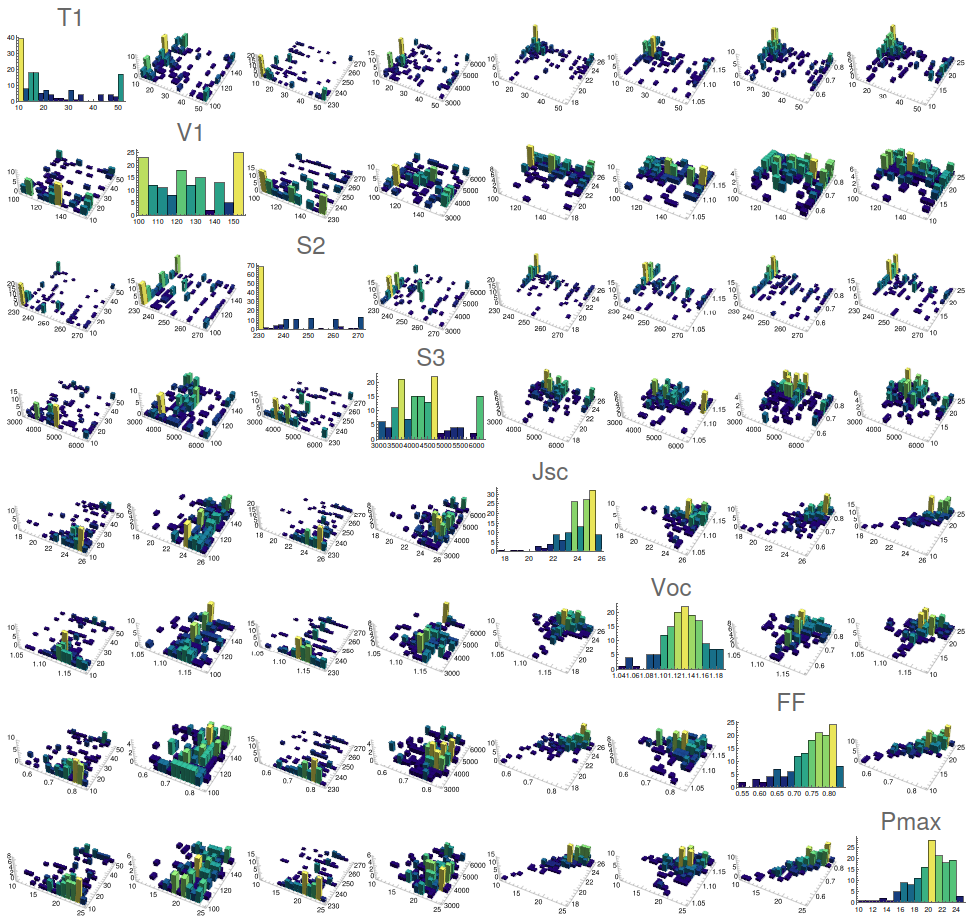
For starters, one of the most elemental descriptions of the datasets corresponds to a global study of its distribution, which can be done via 1D histograms. For that, the function YWhistograLL["file.csv"] returns all the formatted histograms for the available numerical variables in a given dataset:

YWhistograLL[wen_String] :=
 Module[{info, tou, hist, se}, info = Import[wen]; tou = info[[1]]; 
  info = Rest[info]; se = ColorData[97, "ColorList"]; 
  hist = Table[
    Histogram[info[[All, i]], PlotLabel -> tou[[i]], 
     PlotTheme -> "Detailed", 
     ChartStyle -> se[[Mod[i, Length[se], 1]]]], {i, Length[tou]}]; 
  Grid[Partition[hist, UpTo[5]], Spacings -> {1, 1}]]

A limit of five histograms per row has been included for better display, and the colour scheme just enables easier identification within the column numbers, but the header is also shown on the top part of the subfigures. When running this code for the three datasets mentioned before:

YWhistograLL["energy.csv"]
YWhistograLL["abalone.csv"]
YWhistograLL["niox.csv"]

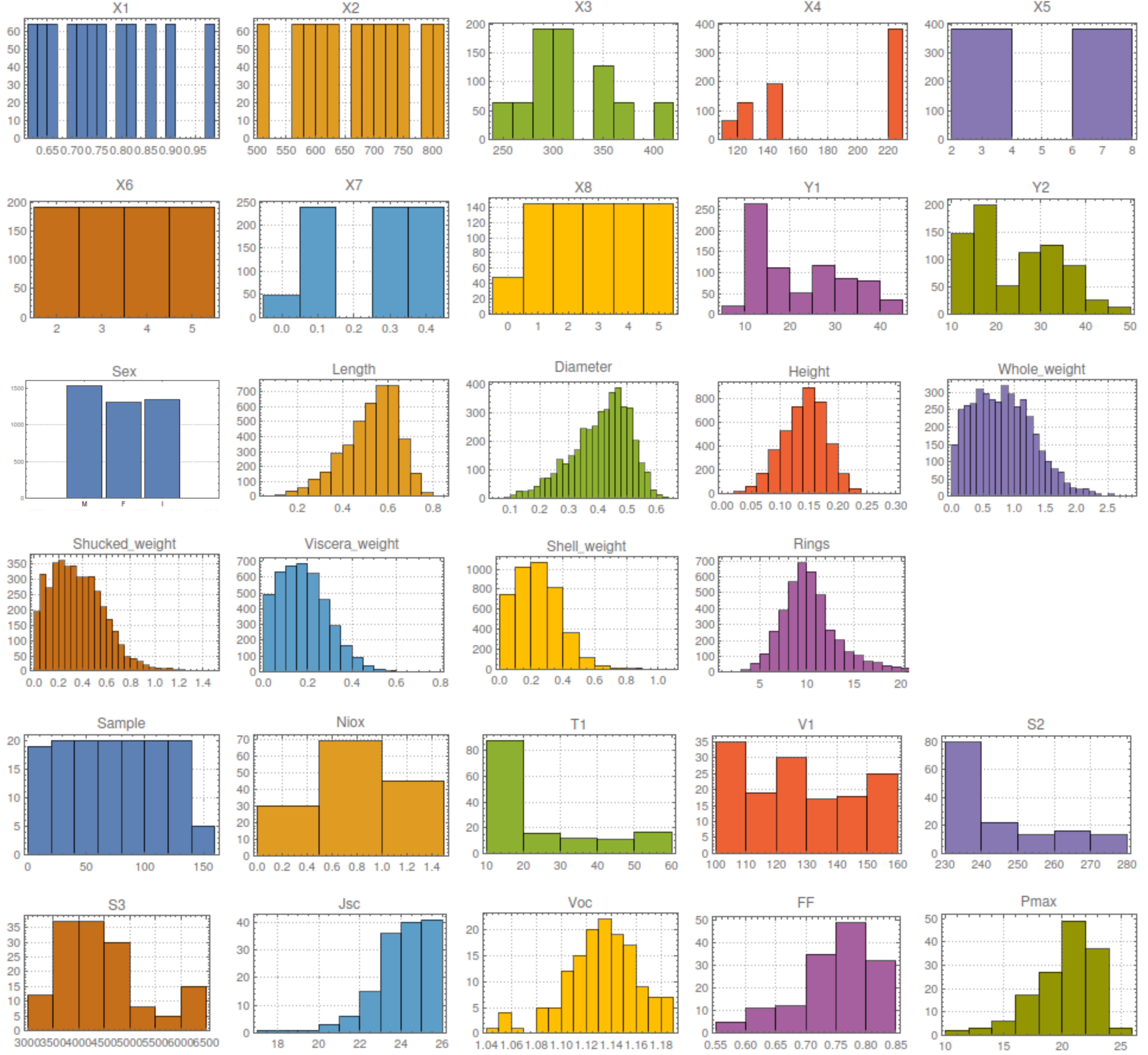
With this simple tool, it is possible to understand some basic properties of the data, including dummy variables and initial apparent correlations between variables. For example, in the case of the buildings, X1-X8 can be identified as inputs, while Y1-Y2 corresponds to the outputs, with a non-trivial correlation between the heating and cooling loads, observing the uniform spread of several features. For its part, in the case of the snails, it is possible to appreciate the asymmetric spread of the variables, corresponding to Poisson/Weibull-like distributions, while for the perovskites cells, it is seen that there are special sub-areas from the global parameter space more explored, while output variables FF and Pmax, exhibit similar trends.

A possible next step is then to start considering the correlations between individual variables, and for that, joint 2D histograms can be a suitable tool. To that end, the function YWdoubLLe["file.csv", variableA,variableB,bins_number]enable to compare the joint histograms of variables A and B, and present them using a tunable amount of bins:

YWdoubLLe[wen_String, varA_Integer, varB_Integer, bin_Integer] := 
  Module[{info, tou, datA, datB, plot}, info = Import[wen];
   tou = info[[1]];
   info = Rest[info];
   datA = info[[All, varA]];
   datB = info[[All, varB]];
   plot = 
    Histogram3D[Transpose[{datA, datB}], {bin, bin}, 
     AxesLabel -> {tou[[varA]], tou[[varB]], "Freq."},
     TicksStyle -> Directive[FontSize -> 18], 
     LabelStyle -> Directive[FontSize -> 18],
     ColorFunction -> "BlueGreenYellow", ColorFunctionScaling -> True,
      ImageSize -> Large,
     PlotTheme -> "Detailed", Boxed -> False, FaceGrids -> None,
     ChartElementFunction -> 
      ChartElementDataFunction["ProfileCube", "Profile" -> 1., 
       "TaperRatio" -> 0.9]];
   plot];

While the last element is purely aesthetic, with this tool we are able to understand better the ideas mentioned before. For example, in case of evalutating it for the case of the building's energy efficiency:

{YWdoubLLe["energy . csv", 2, 9, 15], 
 YWdoubLLe["energy . csv", 6, 8, 18], 
 YWdoubLLe["energy . csv", 9, 10, 20]}

it can be observed that, in general, there exists an inverse relation between the surface area of the building and its efficiency (Fig. 2, left), that apparently the orientation has a weaker correlation with the cooling load (Fig. 2, centre), or that heating and cooling procedures are quite correlated (Fig. 2, right). A similar treatment can be done for the snail case:

{YWdoubLLe["abalone . csv", 5, 7, 60], 
 YWdoubLLe["abalone . csv", 4, 9, 18], 
 YWdoubLLe["abalone . csv", 5, 9, 60]}

where the relation between total weight and gut weight is observed (Fig. 3, left), a diffuse central correlation is observed for height of the animal (Fig. 3, centre) including a couple of outliers, and a more diffuse correlation between total weight and age (Fig. 3, right), as mentioned before. Finally, for the case of the perovskite experimental characterisation:

{YWdoubLLe["niox . csv", 1, 2, 18], 
 YWdoubLLe["niox . csv", 4, 6, 18], 
 YWdoubLLe["niox . csv", 9, 10, 18]}

it is found that the optimisation process lead towards intermediate values of NiOx concentration (0.5, Fig. 4 left), highlighting of the apparent independence between feature input variables such as CB volume and high spin speed V1-S3 (Fig. 4, centre) and a notable correlation (above the other outputs, Jsc and Voc) between FF and Pmax (Fig. 4, right). The question now is whether is possible to perform all the combinations at once, to understand the matrix of correlations or pair-wise dependencies and enables a global understanding of the basic relations underlying two variables. A possible implementation [I], with similar syntax as the previous case, could be the following:

YWcorreLLation[wen_String, vars_List, bins_Integer] := 
 Module[{info, tou, data, n, plots}, info = Import[wen];
    tou = info[[1]];
    data = Rest[info];
    n = Length[vars];
    plots = 
   Table[If[i == j, 
     Histogram[data[[All, vars[[i]]]], bins, 
      PlotLabel -> Style[tou[[vars[[i]]]], FontSize -> 36], 
      ChartStyle -> "BlueGreenYellow", 
      ColorFunction -> 
       Function[{heights}, ColorData["BlueGreenYellow"][heights]], 
      ColorFunctionScaling -> True, ImageSize -> Small], 
     Histogram3D[
      Transpose[{data[[All, vars[[i]]]], 
        data[[All, vars[[j]]]]}], {bins, bins}, 
      ColorFunction -> "BlueGreenYellow", 
      ColorFunctionScaling -> True, ImageSize -> Small, 
      PlotTheme -> "Detailed", Boxed -> False, 
      FaceGrids -> None]], {i, n}, {j, n}];
    Grid[plots, Spacings -> {0, 0}]]

Then, the previous cases can be seen just as elements of the general matrix, and where the diagonal elements correspond to the singular histograms, and with symmetry across the diagonal corresponding to the exchange of roles between variables A and B, generalising the results from [E].

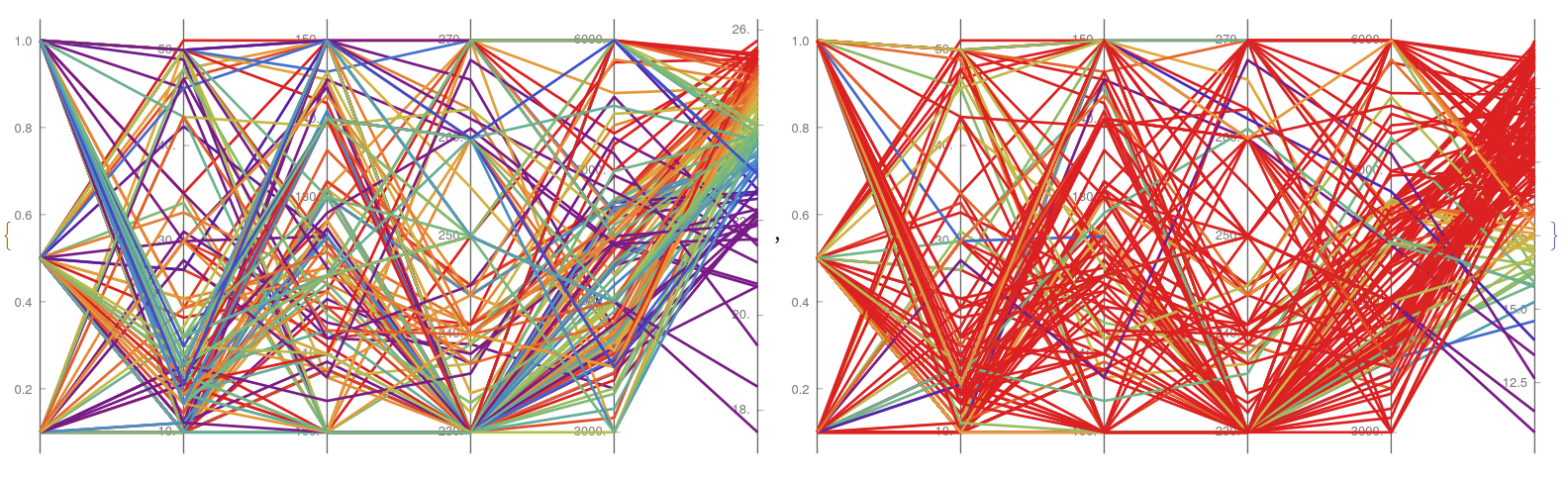
YWcorreLLation["energy . csv", {1, 2, 3, 4, 5, 6, 7, 8, 9, 10}, 6]

Several general features can be seen then on-the-fly; from similar performance against Y1 and Y2, to the minor relative importance of X6 (orientation) or dyadic behaviour of X4 (roof area). Mutatis mutandi with the abalone species:

YWcorreLLation["abalone . csv", {2, 3, 4, 5, 6, 7, 8, 9}, 30]

It is clear that the weight variables are heavily correlated between them, while the diameter and length seems to have a concave relation, while the height seems to include a couple of mutations that opaques the visualisation. Finally, for the perovskite experiment the corresponding syntax would be:

YWcorreLLation["niox . csv", {3, 4, 5, 6, 7, 8, 9, 10}, 15]

It can be seen that corresponds to the most non-linear case, and it is difficult to draw preliminary results from the displayed data. It is surprising, for example, the gaps found in dispense speed (S2), or the apparent preference lines for the dropping volume, that will be explored later. As a generalisation, a three-variable (and higher hyper-)cubic matrix could be also implement in search for 3-correlations in the shape of scatter 3-histograms.

---

Higher dimension pseudo-visualisations

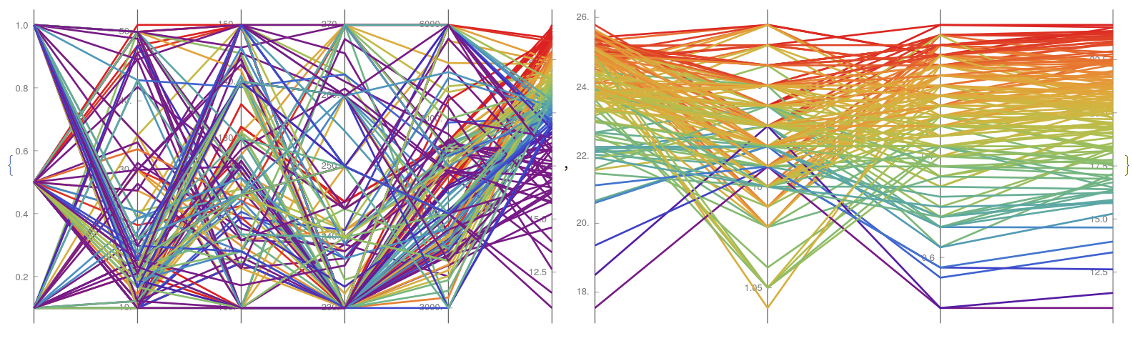
Once the basic visualisation ideas has been tested is worth to use pseudo visualisation where some dimensions lose their spatial degree of freedom and are transformed to parallel display or color scheme. The first tool to be introduced correspond to the parallel coordinates plot [J] popularised in the eighties by A. Inselberg from IBM in parallel (again) with the rise of the personal computers, while technically known almost a century before. There, a single bi-dimensional graph is used to plot all the variables. While the vertical axis show indeed the corresponding values, the horizontal axis is divided in a discrete number of points corresponding to the total number of variables. In this way, the important information is the path that a single line follows, that can characterise the linearity of the model or further correlations. For the implementation, the function:

YWparaLLel["file.csv", variables,variable_colour,range] enables to draw all the trajectory lines and use the last one for a color scale that is modified between the percentiles indicated in the range to better understand the output variables:

YWparaLLel[wen_String, var_List, wei_List] :=
  Module[{info, umbrella, fun, minC, maxC},
   info = Import[wen]; 
   umbrella = info[[2 ;;, var]]; {minC, maxC} = wei;
   fun = 
    ParallelAxisPlot[umbrella, Axes -> True, GridLines -> Automatic, 
     PlotStyle -> Thick,
     ColorFunction -> (ColorData["Rainbow"][
         Rescale[Last[{##}], {minC, maxC}]] &), 
     PlotLegends -> False]];

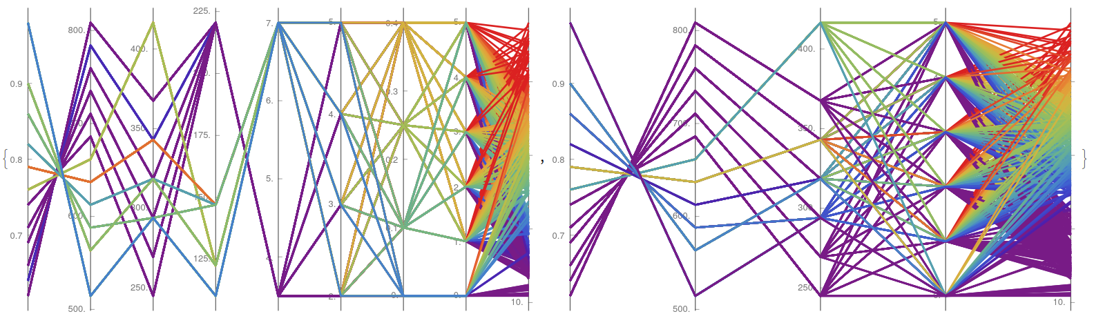
For example, all the input variables (X1-X8) from the building energetic efficiency can be computed (Fig. 8, left) to appreciate the discrete nature of the dataset, while also observing the inverse relation between X1 and X2 (relative compactness and surface area) or the symmetric contribution (preference for intermediate results) in the surface area for a higher heating loading (Y1). This is appreciated further when a simplified case is plotted (Fig. 8, right) display this preference when using a color scale bounded between the third and the ninth decile, while showing with more detail the apparent indifference of parameter X8 (glazing area distribution) towards its efficiency.

{YWparaLLel["energy.csv", {1, 2, 3, 4, 5, 6, 7, 8, 9}, {0.1, 0.8}], 
 YWparaLLel["energy.csv", {1, 2, 3, 8,  9}, {0.3, 0.9}]}

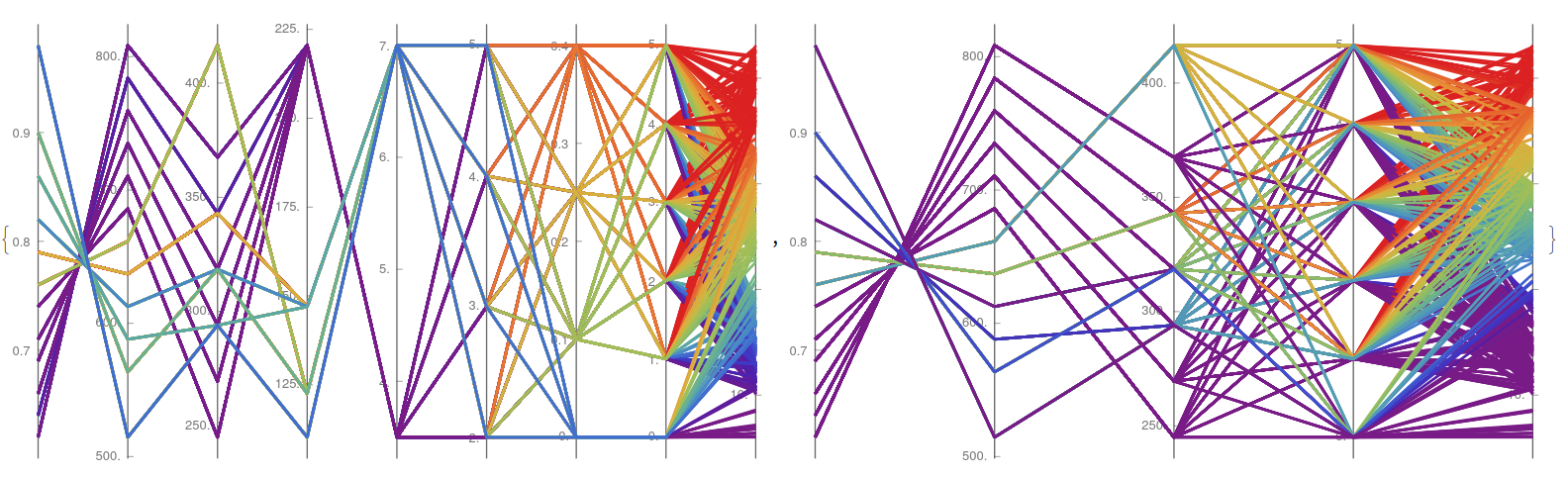
Furthermore, it is possible to replicate these results with the corresponding cooling loading (Y2), to see almost identical trends, with the exception of the relative importance of the roof area (X4) that shows lighter color lines, meaning than its impact on the heating is more relevant than in the cooling one.

{YWparaLLel["energy.csv", {1, 2, 3, 4, 5, 6, 7, 8, 10}, {0.1, 0.8}], 
 YWparaLLel["energy.csv", {1, 2, 3, 8, 10}, {0.3, 0.9}]}

A similar procedure can be done for the dataset corresponding to the snails, in which the most of the variables have a positive correlation, with almost parallel lines, while the cases of meat and dried shell shows some exceptions, as older species seem to slowly lose weight while aging.

YWparaLLel["abalone.csv", {1, 2, 3, 4, 5, 6, 7, 8, 9}, {0.05, 0.95}]

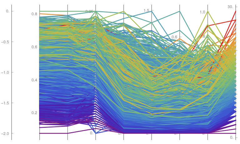
When removing the partial weights (Fig. 11, left), this shrinking becomes more obvious while the diameter seems to be a less fragile measure. In parallel, when studying all the weights independently (Fig. 11, right), it is seen that those quantities are proportional one to the others, with minor exceptions for the meat and guts, with a net transfer from one group to the other; further statistics could be performed to see whether this is a sexual dependent feature, or appear during the initial years of the animal species.

{YWparaLLel["abalone.csv", {2, 3, 5, 9}, {0.15, 0.85}], 
 YWparaLLel["abalone.csv", {6, 7, 8, 5}, {0.15, 0.85}]}

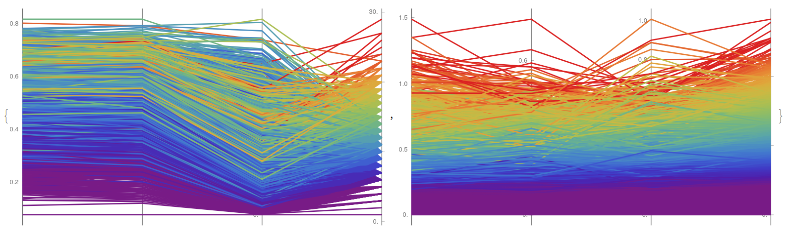
Finally, using this tool for the perovskite experiment, it is possible to showcase the highly non-linear behaviour of the dataset in the case of measuring the Jsc (Fig. 12, left), this is later show in the detailed figure (Fig. 12, right), where the cases between second and sixth decile practically cover all the experimental range of the platform.

{YWparaLLel["niox.csv", {2, 3, 4, 5, 6, 7}, {0.6, 0.95}], 
 YWparaLLel["niox.csv", {2, 3, 4, 5, 6, 10}, {0.2, 0.6}]}

To understand further these relations, the Pmax value is also highlighted (Fig. 13, left) observing that it offers a more condensed distribution of parameters, as the whole space appears more pale, meaning that the region of interest is smaller, what favours further detailed exploration. Finally, the comparison among all the experimental outputs on the performance of the solar cells (namely Jsc, Voc, FF, and Pmax, noticing that Pmax is the product of the previous) illustrate a closer agreement between FF and Pmax, while suggesting that Voc is the most unstable measurement for successful technological applications.

{YWparaLLel["niox.csv", {2, 3, 4, 5, 6, 10}, {0.6, 0.95}], 
 YWparaLLel["niox.csv", {7, 8, 9, 10}, {0, 1}]}

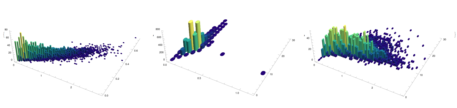
Now that a spatial independent representation is presented it is worth to reconsider more meaningful spatial reconstructions where three variables are used to display a scatter plot of points whose colour represent a fourth variable and its relative size can be used to represent a fifth one, typically one corresponding to the output measurements. For the representation of these spheres, the function:

YWbaLL["file.csv", x-variable, y-variable, z-variable, colour-variable, radius-variable] offers a valuable pseudo-plot with up to five dimensions involved, that can further complemented with coloured or pattered lines in the surface of the sphere to characterise different population sets. In particular, using a non-linear function for the radius turns out to be use for highlighting maximal points in an optimisation process by using a exponential growth close to the theoretical limit.

YWbaLL[wen_String, x_Integer, y_Integer, z_Integer, c_Integer, 
  r_Integer] := 
 Module[{info, xx, yy, zz, cc, rr, p, colorFunction, mainPlot, 
   legend}, info = Import[wen];
  xx = info[[2 ;;, x]]; yy = info[[2 ;;, y]]; zz = info[[2 ;;, z]];
  rr = info[[2 ;;, r]]; cc = info[[2 ;;, c]];
  rr = 0.015 + 0.01/(Max[info[[2 ;;, r]]] + 0.05 - info[[2 ;;, r]]);
  xx = Rescale[xx]; yy = Rescale[yy]; zz = Rescale[zz]; 
  cc = Rescale[cc];
  colorFunction = ColorData["AvocadoColors"];
  p = Table[
    Graphics3D[{EdgeForm[], 
      Style[Sphere[{xx[[i]], yy[[i]], zz[[i]]}, rr[[i]]], 
       colorFunction[cc[[i]]]]}], {i, 1, Length[xx]}];
  mainPlot = 
   Show[p, Axes -> True, 
    AxesLabel -> {"Var" <> ToString[x], "Var" <> ToString[y], 
      "Var" <> ToString[z]}, Boxed -> False, ImageSize -> Large, 
    PlotRange -> All, Lighting -> "Accent"];
  legend = 
   BarLegend[{colorFunction, {Min[cc], Max[cc]}}, 
    LegendLabel -> "Var" <> ToString[c]];
  Row[{legend, Spacer[10], mainPlot}]]

This is basically a normalised scatter plot in three dimensions but with two additional degrees of freedom, one corresponding to the colour scale and the other to the size of the radius. A output/target variable can be use in any of them, but in this case it is typically used in the radial variable, to include non-linearities that favours the understanding of the relevant manifolds. This way it is possible to get a better understanding of multidimensional data. For example:

{YWbaLL["energy.csv", 3, 8, 1, 6, 9], 
 YWbaLL["energy.csv", 8, 7, 2, 6, 9]}

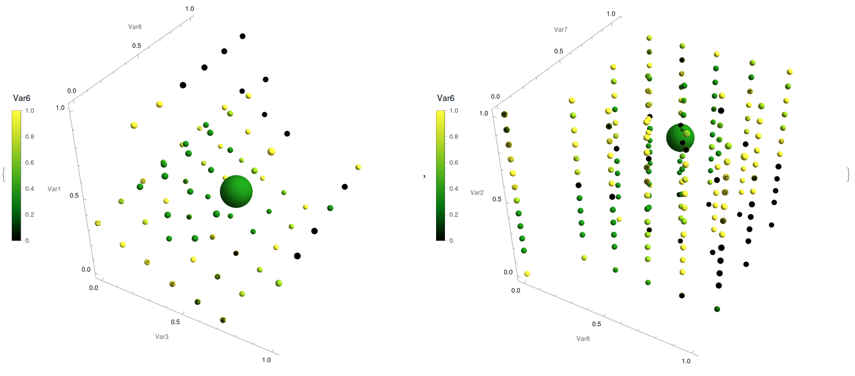
With this analysis is easy to spot that it is favourable to aim towards average values of compactness or wall area (Fig. 14, left) while aiming towards higher values of glazing area (Fig. 14, right) is one wants to maximise the loading. In the case of the snails:

{YWbaLL["abalone.csv", 2, 3, 4, 5, 9], 
 YWbaLL["abalone.csv", 6, 7, 8, 5, 9]}

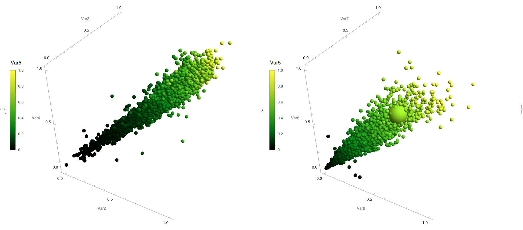
Enables, for its part, to unveil a direct positive general correlation between length, diameter, height, and age (Fig. 15, left) while for the interdependencies on the different weights, it is seen that there is a stationary weight than older species tend to, corresponding to a decrease from adult numbers. Finally, for the solar cell case:

{YWbaLL["niox.csv", 3, 4, 5, 6, 10], 
 YWbaLL["niox.csv", 7, 8, 9, 6, 10]}

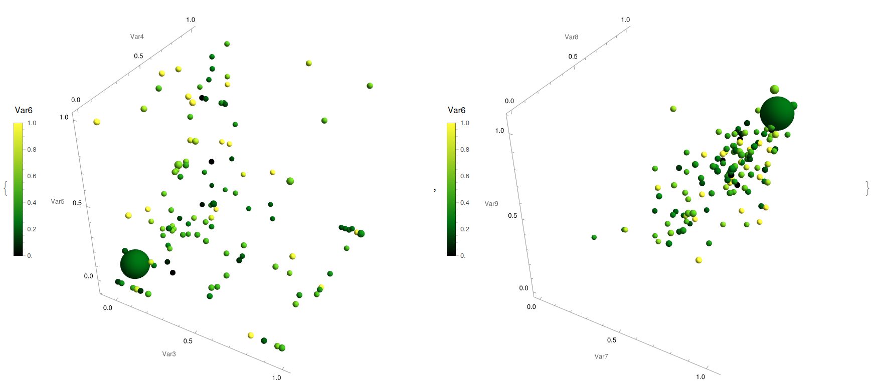
It can be appreciated again the non-linear nature of the cloud of points while appreciating the restrictive experimental parameter space as there is a overload towards lower values on the machine selected area, with the maximal cases situated close to a corner (Fig. 16, left). Also, the different physical measurements for characterising the solar cell efficiency are displayed together, with its distance to the origin (in particular, its product) is proportional to the radius displayed, observing some anomalies far from a linear positive dependence.

Overall, we have now introduced how to represent existing multidimensional datasets in a compact display, but without generating any additional information from them. In the next section, a weakly stochastic gradient descent simple model, umbrella model, is introduced to suggest new experimental points to try looking for higher values of the output / target variables, like in perovskite solar cell optimisation or in building's energetic efficiency.

---

Prediction models

The problem of optimisation and search for global minima and maxima of arbitrary functions is still an open question in terms on computational complexity. While convex properties enable a simplified global-local correspondence, the existence of a general case parameter-free algorithm is still unknown. In the case of discrete set of evaluations, such as experimental scenarios, classic gradient descent based on finding directions of maximum growth (or decrease, if the objective is to minimise a cost function, for example) gives surprisingly good results when properly adapted. For example, adding stochastic noise to the solutions enables a higher cross section and clash with extremes.

In the previous multidimensional (but still reasonable, with less than 10 dimensions) cases, the studied inputs gives a set of initial vectors (input) that evaluated in the theoretical function returns another vector of target functions (outputs). In the examples shown above, the heat loading values, age of the abalone species or power conversion efficiency for perovskite solar cells is found to be the objective to maximize. Here, we suggest a simple analytical algorithm, strongly based on gradient descent that aims to offer new experimental parameter sets to test.

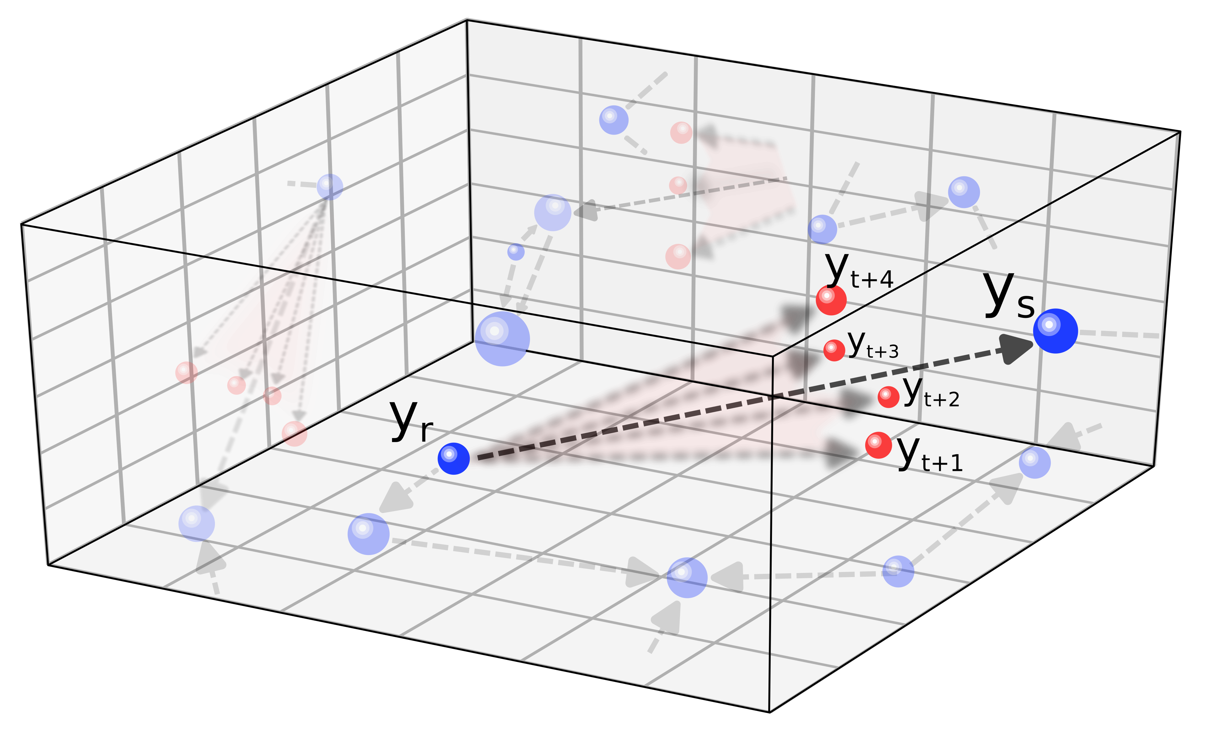
Mathematically, a vector y of input parameters are renormalised to the [0,1] interval using an Euclidean metric. Later, among the vicinity of each point, the surrounding gradients are computed and ranked, according to the values of||f(Subscript[y, s])-f(Subscript[y, r])||/(Subscript[y, s]-Subscript[y, r]). Later, a new batch of experimental realisation is suggested following the expression Subscript[y, t]=(1+[Eta])Subscript[y, r]+[PlusMinus][Alpha](Subscript[y, s]-Subscript[y, r]), where [Eta] correspond to a numerical noise (Gaussian~ N(0,[Sigma]^2), in the case below) that enables a higher probability of extrema finding in non-linear landscapes, and [Alpha] is a unitary parameter that represent the relative position of the new set of points with respect to the initial and final point of the selected gradient. In the case of close to the unity values, the overall picture loosely resemble to the figure of a (almost closed) umbrella, and inspired the labelling of it.

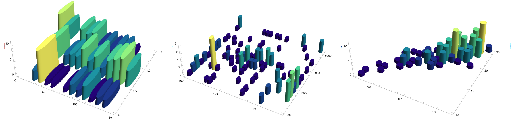
Then, a possible implementation of this idea can be found below within the function:

YWbaLL["file.csv", inputlist, outputvariable, plotting_options, neighbours, [Alpha], [Sigma]], corresponding to a f(inputs)=output schema, unfortunately only valid of a single output variable, although a composed function of several parameters can be defined, and the corresponding plotting options and numerical conditions, such as local environment to search the gradients, or noise. From there, the gradients are computed and ranked, to later compute different set of new points. In green (in the code MM), intermediate points corresponding to the top gradients, to discard or explore intermediate extrema; in red (in the code LR), the corresponding umbrella candidates, and finally in blue (in the code CC) some sanity check cases around the current maxima. Finally, those new candidates to test and evaluate its performance are exported in the same format as the input file to continue the exploring procedure.

YWumbreLLa[wen_String, in_List, out_List, plt_List, n_, alpha_, 
  sigma_] :=
 Module[{info, input, output, 
   rank, \[Alpha], \[Eta], \[Sigma], \[CapitalDelta],
   normu, euclu, nearu, gradu, topgradu, ninput, noutput, nn, 
   nnoutput, topout, scalu,
   tryMM, tryLR, tryCC, xx, yy, zz, cc, size, p00, pMM, pLR, pCC, exp,
    lim, w, ww},
  info = Import[wen]; info = Rest[info]; 
  input = Transpose[info[[All, in]]];
  output = Transpose[info[[All, out]]][[1]]; 
  rank = n; \[Alpha] = alpha; \[Sigma] = sigma;
  normu[vec_] := (vec - Min[vec])/(Max[vec] - Min[vec]);
  euclu[p1_, p2_] := Sqrt[Total[(p1 - p2)^2]];
  ninput = Map[normu, input]; 
  noutput = Transpose[Append[ninput, output]];
  nearu[info_] := Module[{dd, nn}, dd = Table[If[i == j, 1000,
       euclu[info[[i, 1 ;; -2]], info[[j, 1 ;; -2]]]], {i, 
       Length[info]}, {j, Length[info]}];
    nn = Map[First@*Ordering, dd, {1}]; nn];
  nnoutput = nearu[noutput];
  gradu = Table[Module[{outid, dd, delta}, outid = nnoutput[[i]];
     dd = euclu[noutput[[i, 1 ;; -2]], noutput[[outid, 1 ;; -2]]];
     If[dd == 0, dd = 10^10];
     delta = Abs[noutput[[i, -1]] - noutput[[outid, -1]]]/dd;
     delta], {i, Length[noutput]}];
  topgradu = Ordering[gradu, -rank];
  \[Eta] = RandomReal[NormalDistribution[0, \[Sigma]]];
  tryMM = Table[Module[{id, outid, MM}, id = topgradu[[i]];
     outid = nnoutput[[id]];
     MM = (noutput[[id, 1 ;; -2]] + noutput[[outid, 1 ;; -2]])/
        2*(1 + \[Eta]);
     MM], {i, rank}];
  tryLR = Table[Module[{id, outid, LR, grad}, id = topgradu[[i]];
     outid = nnoutput[[id]];
     grad = noutput[[outid, 1 ;; -2]] - noutput[[id, 1 ;; -2]];
     If[noutput[[outid, -1]] > noutput[[id, -1]],
      LR = noutput[[outid, 1 ;; -2]] + \[Alpha]*grad*(1 + \[Eta]),
      LR = noutput[[outid, 1 ;; -2]] - \[Alpha]*grad*(1 + \[Eta])];
     LR], {i, rank}];
  scalu[vec_, zero_] := vec*(Max[zero] - Min[zero]) + Min[zero];
  tryMM = 
   Transpose[
    Table[scalu[tryMM[[All, j]], input[[j]]], {j, Length[input]}]];
  tryLR = 
   Transpose[
    Table[scalu[tryLR[[All, j]], input[[j]]], {j, Length[input]}]];
  topout = First[Ordering[info[[All, Last[out]]], -1]];
  nn = nnoutput[[topout]];
  \[CapitalDelta] = info[[nn, in]] - info[[topout, in]];
  tryCC = If[info[[nn, Last[out]]] > info[[topout, Last[out]]],
    info[[nn, in]] + \[Alpha]*\[CapitalDelta] (1 + \[Eta]),
    info[[nn, in]] - \[Alpha]*\[CapitalDelta] (1 + \[Eta])];
  xx = plt[[1]]; yy = plt[[2]]; zz = plt[[3]]; cc = plt[[4]];
  w = If[FileExistsQ[info], First[Import[info]], {}]; size = 0.006;
  ww = Table[
    If[Length[w] >= in[[i]], w[[in[[i]]]], 
     StringJoin["Var", ToString[in[[i]]]]], {i, Length[in]}];
  p00 = ListPointPlot3D[{Table[{input[[xx, i]], input[[yy, i]], 
       input[[zz, i]]},
      {i, 1, Length[input[[1]]]}]}, 
    PlotStyle -> Directive[Black, PointSize[size]]];
  pMM = ListPointPlot3D[{Table[{tryMM[[i, xx]], tryMM[[i, yy]], 
       tryMM[[i, zz]]},
      {i, 1, Length[tryMM]}]}, 
    PlotStyle -> Directive[Green, PointSize[2.5*size]]];
  pLR = ListPointPlot3D[{Table[{tryLR[[i, xx]], tryLR[[i, yy]], 
       tryLR[[i, zz]]},
      {i, 1, Length[tryLR]}]}, 
    PlotStyle -> Directive[Red, PointSize[2.25*size]]];
  pCC = ListPointPlot3D[{{tryCC[[xx]], tryCC[[yy]], tryCC[[zz]]}},
    PlotStyle -> Directive[Blue, PointSize[2.75*size]]];
  Print[Show[p00, pMM, pLR, pCC, ImageSize -> Large,
    Boxed -> True, BoxRatios -> {1, 1, 1}, Axes -> True, 
    AxesLabel -> {ww[[xx]], ww[[yy]], ww[[zz]]}]];
  exp = DeleteDuplicates[Join[tryMM, tryLR, {tryCC}]];
  w = If[FileExistsQ[info], First[Import[info]], {}];
  ww = If[Length[w] > 0, w[[in]], 
    Table[StringJoin["Input", ToString[i]], {i, Length[in]}]];
  Export[
   StringJoin["samples_", DateString[{"Month", "Day"}], ".csv"],
   Prepend[Append[#, ""] & /@ exp, ww]]; Return[Null]; ]

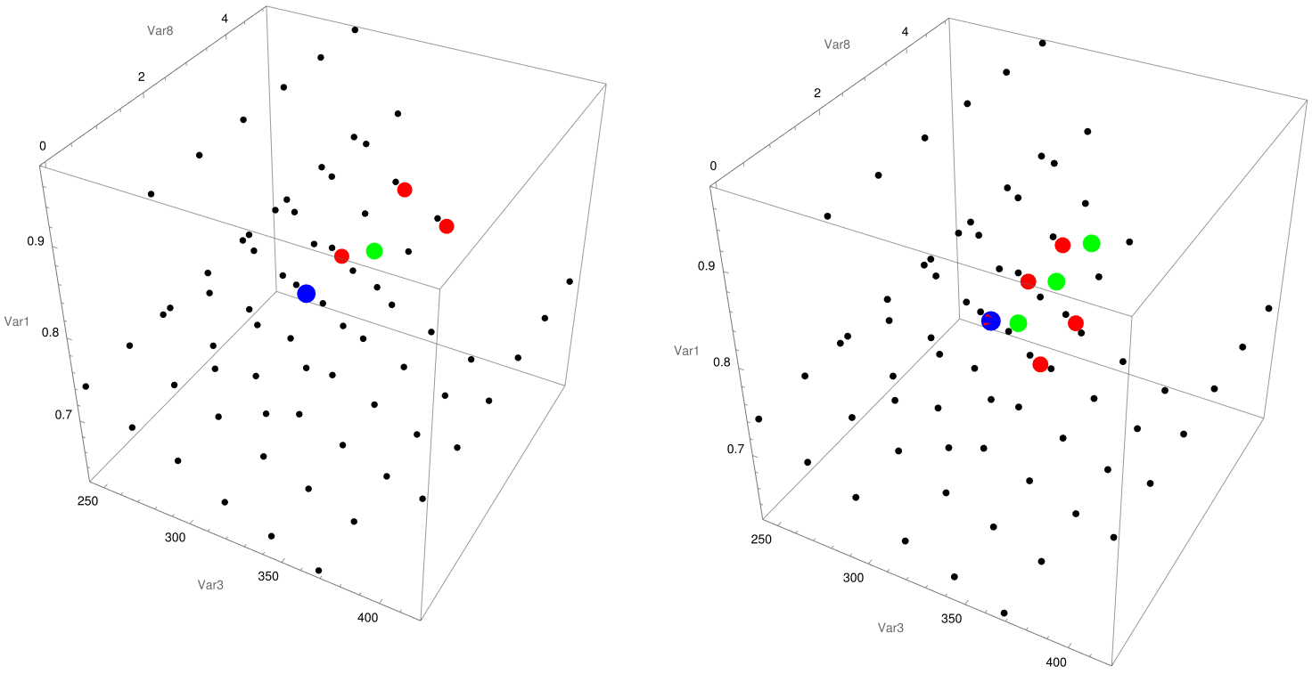
Examples of its implementation can be found below for the three tested dataset, where a greater environment is explorer, and then more points are suggested for both heating and cooling loadings:

{YWumbreLLa["energy.csv", {1, 2, 3, 4, 5, 6, 7, 8}, {9}, {3, 8, 1, 6},
   3, 0.2, 0.1], 
 YWumbreLLa[
  "energy.csv", {1, 2, 3, 4, 5, 6, 7, 8}, {10}, {3, 8, 1, 6}, 5, 0.2, 
  0.1]}

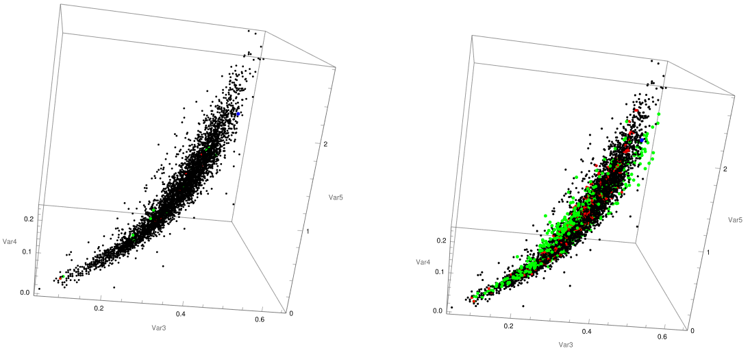
For its, part the visualization tools enable to explore the distribution of the new suggested points under different diagrams:

{YWumbreLLa["abalone.csv", {2, 3, 4, 5}, {9}, {2, 3, 4, 5}, 20, 0.5, 
  0.1], YWumbreLLa["abalone.csv", {2, 3, 4, 5}, {9}, {6, 7, 8, 5}, 
  500, 0.5, 0.1]}

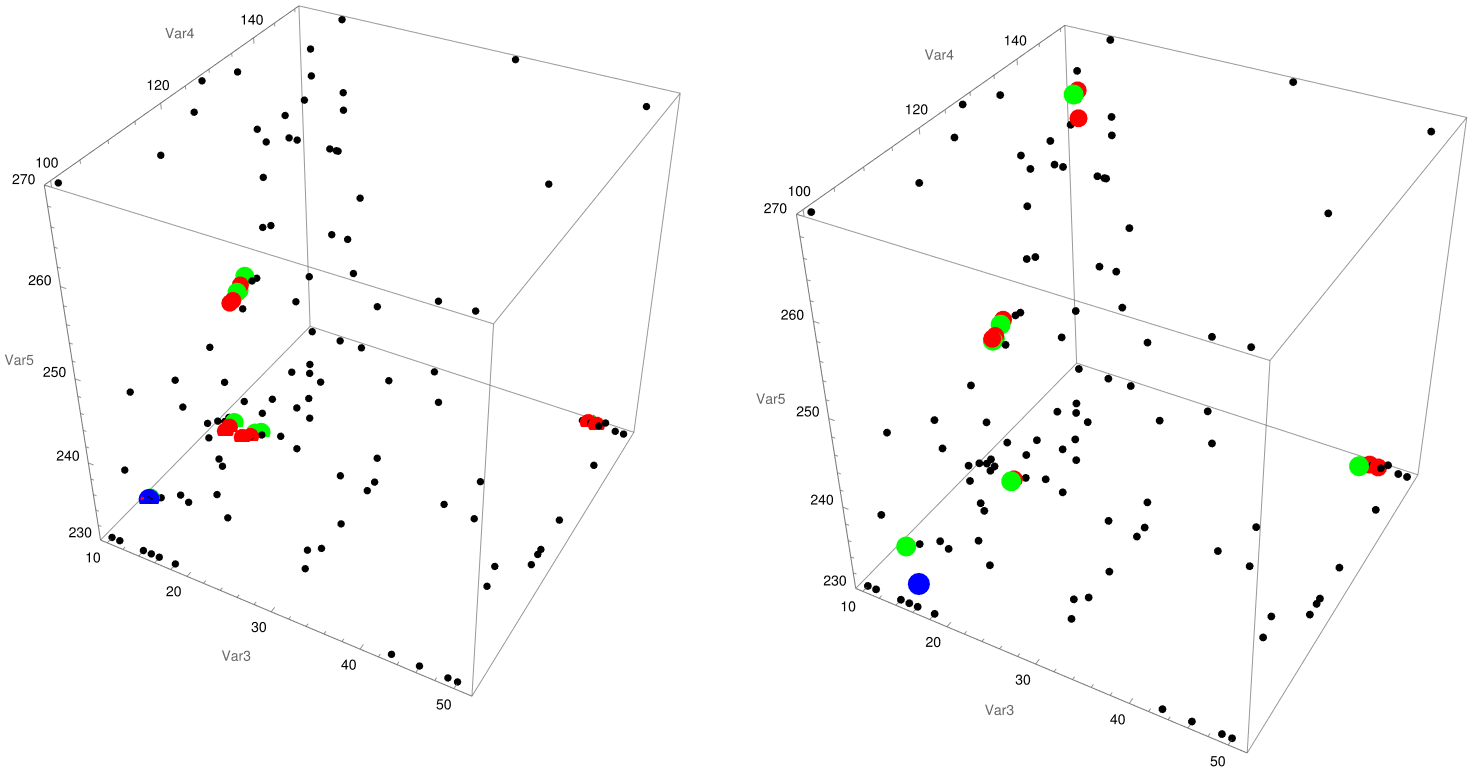
Finally, the increase in the noise of the prediction model can be arbitrarily tuned under the value of the parameter [Sigma] to find a suitable trade off between exploration and exploitation, and control the deterministic aspect of the algorithm:

{YWumbreLLa["niox.csv", {2, 3, 4, 5, 6}, {10}, {2, 3, 4, 5}, 20, 0.7, 
  0.05], YWumbreLLa["niox.csv", {2, 3, 4, 5, 6}, {7}, {2, 3, 4, 5}, 
  20, 0.7, 0.2]}

---

Discussion

This work presented the LLOVE toolbox within the Mathematica environment that can be use for fast testing and modelling in the realm of multidimensional data analysis and visualization. This suite of tools addresses a growing need for more intuitive and accessible methods to explore complex datasets, particularly between the fields where traditional visualization techniques fall short, and high-dimension spaces where machine learning techniques find suitable dimensional compression. The initial suite of visualisation tools (histograLL, doubLLe, and correLLAtion), provides students and researchers a initial exploratory tool to evaluate some correlations within their datasets that might otherwise remain hidden in raw data, without introducing any novel idea that could restrict to use these functions on a elementary level.

The introduction of pseudo-visualization techniques, such as paraLLel coordinates plots and five-dimensional scatter plots, offers the next step in complexity, providing a simple tool to test roughly linearities. Finally, the umbreLLa model, based on a stochastic gradient descent approach, offers a complementary tool for retrieving unexplored areas in optimisation scenarios. By incorporating noise into the gradient descent process, the model effectively balances exploration and exploitation, increasing the likelihood of identifying global extrema.

Without limiting to the previous examples but with a particular interest on applying to the solar cell community [L], we believe this suite could be useful for a general research profile. Next steps aim towards further tools development, accessibility and UI implementation, and online web availability without any installation of software, priorities in the development on future versions of the package LLOVE in the Wolfram language.

---

Acknowledgments

Y.W acknowledges support from ERC C2C-PV Grant No. 101088359. S.P.P. acknowledges support from the SALTO program (MPG/CNRS) No. 57142201151. The authors declare no conflicts of interest regarding this manuscript.

---

Bibliography

[A] A.C. Heusser, K. Ziman, L. L. W. Owen, J.R. Manning (2017) HyperTools: A Python toolbox for visualizing and manipulating high-dimensional data.

[B] C. Drozdowski (2018)Origin 2019 Introduces Parallel Plots.

[C] MathWorks Inc. (2025) Visualizing Four-Dimensional Data.

[D] Wolfram Inc. (2024) High-Dimensional Visualization.

[E] A. Tsanas and A. Xifara (2012) Accurate quantitative estimation of energy performance of residential buildings using statistical machine learning tools. Energy and Buildings 49 560-567.

[F] W. Nash, T. Sellers, S. Talbot, A. Cawthorn, and W. Ford (1995) Abalone: Predicting the age of abalone from physical measurement.

[G] Y.Wang et. al. (2024) Hybrid learning enables reproducible >24% efficiency in autonomously fabricated perovskites solar cells, manuscript under publication.

[H] W. J. Nash, T. L. Sellers, S. R. Talbot, A. J. Cawthorn, and W. B. Ford (1994) The Population Biology of Abalone (Haliotis species) in Tasmania. I. Blacklip Abalone (H. rubra) from the North Coast and the Islands of Bass Strait. Technical Report 48, ISSN 1034-3288.

[I] For example, in Mathematica, the function PairwiseDensityHistogram do a similar function, as the projection in the plane of the bidimensional histograms is meaningful thanks to the chosen colour scale.

[J] A. Inselberg (1985), The plane with parallel coordinates The Visual Computer 1 69-91.

[K] S.G. Waugh (1995), Extending and benchmarking Cascade-Correlation : extensions to the Cascade-Correlation architecture and benchmarking of feed-forward supervised artificial neural networks Thesis from University of Tasmania.

[L] T.J. Jacobsson, A. Hultqvist, A. García-Fernández, et al. (2022) An open-access database and analysis tool for perovskite solar cells based on the FAIR data principles. Nat Energy 7, 107[Dash]115 (2022).

[K] *https://zenodo.org/records/15870982*